Analyzing Phoenix Yelp Reviews
Introduction
Welcome to this AC209a Data Science project on User Ratings and Reviews. We chose to work with data from the "Yelp Dataset Challenge" [1], which is a huge repository of data about businesses and the users rating them in a variety of formats. This website will walk you through our investigation of it, as we follow the data science process from cleaning to conclusions.
Our project's core focus is on applying recommendation system techniques from the BellKor solution to the Netflix Grand Prize [2] to the Yelp dataset, but we also devoted significant time exploring a number of other techniques -- as well as the data itself.
Data Exploration
The Yelp Challenge dataset is very high-dimensional and split across multiple distinct categories. We chose to focus on just users, businesses without their photos, and reviews without their associated text, though we did a little bit of exploration and brainstorming about text and images. Although the data came fairly cleanly packaged, we did decide to convert it from a nested JSON structure to a flat CSV structure suitable for use in pandas (which we used extensively), and wrote several common scripts to load and augment the data with useful location and time-based features.
The topics we investigated in data exploration can be subdivided into general exploration, location based analysis, network analysis and time based analysis.
After investigating the entire dataset, which spans 10 cities around the globe, we chose to focus our investigation on restaurants and bars in Phoenix, Arizona. The dataset contains many "one review" users (i.e. users that only submit one review); these cases are particularly hard to make predictions for due to a lack of user history. While it is true that Yelp users will occasionally travel between cities, we wanted to limit the scope of our analysis to some subset where there was likely to be a greater overlap between businesses rated by users (i.e. hone the analysis in on one city). Additionally, we chose to limit our study to restaurants and bars as it's more conceivable that users will share preferences within a single category rather than across categories. After limiting the dataset in this manner, the sparsity of the dataset decreased by about an order of magnitude.
Baseline Analysis
The full dataset contains 2,700,000 reviews from 687,000 users for 86,000 businesses. The business dataset consists of 15 features including category of business (e.g., fast food, restaurant, nightlife, etc.), full address, operation hours, latitude, longitude, review count, and stars earned. We augmented it to include the city. The user dataset consists of 11 features including average stars, compliments, elite, number of fans, friend IDs, name, review count, vote categories, and when they started Yelping.
Both the user and business data is highly right skewed. Most users rate only a small number of businesses, and similarly, the majority of businesses receive a comparatively small number of reviews, though less extremely so than users. The implications of this observation for us is that using a particular user's review history to predict that user's rating for any one particular business is likely to be unfruitful (the small user history will prevail for the majority of cases). We run this analysis in Interpretable Linear Models and we see that while including a user's review history does add a useful predictor, it does not dramatically improve the general prediction for most users. However, we did find that once we limited the dataset to users with at least a few reviews, our accuracy improved significantly.
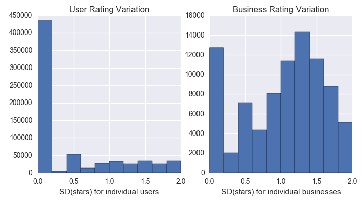
Users tend to rate businesses highly with the ratings between 4 and 5 consisting of a total of 67% of all of the entered reviews in the system. In agreement with this, the users also typically tend to give many similar reviews, as we see that the majority of users have a very small range in the number of stars that they give. In contrast to this, we see that businesses tend to receive a large range of reviews. This speaks to the preferences of individuals - what works for one person might not work for another. The key learning here is that since users tend not to deviate from their review, we can possibly bias a model by using a user's mean rating to that point in time (the caveat here is that this data must exist as noted in the point above). It is also important to note that using a business's mean score may be a poor predictor for individual user's ratings due to the variation in these ratings.
Having decided to explore the culinary experience in Phoenix, and inspired by the homework assignment on movie reviews, we wanted to understand the scope for the best and worst ratings. The problem here is that a restaurant that receives few reviews may have a disproportionately unrepresentative sample. Therefore, considering only the raw business rating would lead to an unreliable result. Similarly, considering only the number of reviews is unintuitive as a business with many low scores cannot be considered a 'good' restaurant. To resolve these issues, we treated our knowledge about the quality of a restaurant probabalistically, modeling our belief in its ranking (from 0 as bad to 1 as great) as a Beta distribution initially centered at 0.5. We treated 5-star reviews as upvotes and 1-star reviews as downvotes, with values in between counting to some degree as both up and downvotes (a technique we applied somewhat successfully again later). A few examples of the rankings that method generated are given in the tables below:
The Highest-Ranked 5 Restaurants in Phoenix
| Name | Categories | Review Count | Avg. Stars |
|---|---|---|---|
| Little Miss BBQ | Barbeque, Restaurants | 944 | 4.794 |
| El New Yorican Central Catering & Delivery | Puerto Rican, Spanish, Caribbean, Restaurants | 139 | 4.855 |
| Top Marks Cafe | Food, Gelato, Coffee & Tea, Creperies | 33 | 5.000 |
| The Local Press Sandwich Bar | Sandwiches, Restaurants | 47 | 4.974 |
| Tacos Chiwas | Mexican, Restaurants | 89 | 4.915 |
The Lowest-Ranked 5 Restaurants in Phoenix
| Name | Categories | Review Count | Avg. Stars |
|---|---|---|---|
| Dairy Queen | Fast Food, Restaurants | 33 | 1.280 |
| Pizza Hut | Italian, Pizza, Chicken Wings, Restaurants | 7 | 1.000 |
| KFC | Fast Food, Chicken Wings, Restaurants | 13 | 1.154 |
| McDonald's | Burgers, Fast Food, Restaurants | 18 | 1.313 |
| Far East Asian Fire | Chicken Shop, Asian Fusion, Restaurants | 25 | 1.211 |
Time Exploration
One of the most successful methods in the BellKor solution to the Netflix challenge involved taking into account various temporal effects present in the data, both over long spans and short intervals. We were interested in exploring whether or not these were effects we'd be able to find in the Yelp data, as well.
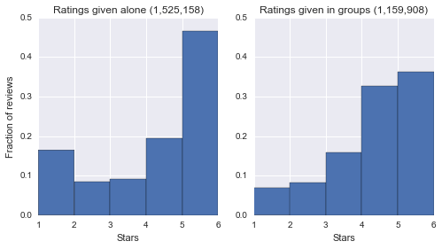
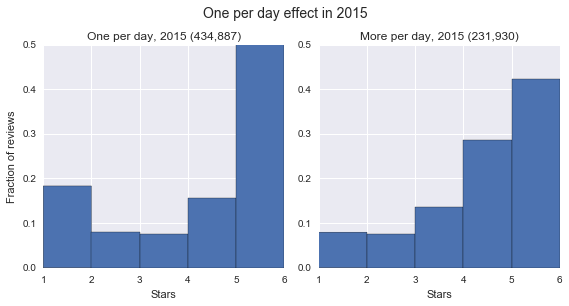
One of the major phenomena cited in [2] was that users who only rate one item on a given day tend to exhibit different behaviors than users rating multiple items. As seen below, we definitely noticed such an effect; users who rate only one item per day tend to be more likely to select 1 or 5. The intuition behind this seems to be that if a user is only giving a single rating, they are likely opening the Yelp app simply because they had a particularly good or bad experience rather than out of a general dedication to rating every business they encounter.
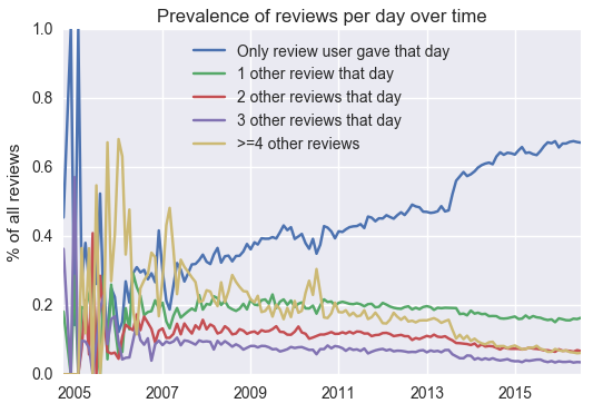
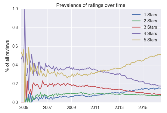
We also noticed that there were some long-term trends in the data. In particular, 1s and 5s have been becoming increasingly prevalent in Yelp for a long time, as have users who only give one review at a time:
It's natural to ask whether the difference in the distribution of ratings between users giving one review per day vs. multiple is causing the change in the distribution of ratings, or vice versa -- perhaps reviews that are given alone on a day are just more likely to be recent, and recent reviews are more extreme overall. However, the effect remains even when conditioning on the year, which suggests that the effect isn't just attributable to the recent past.
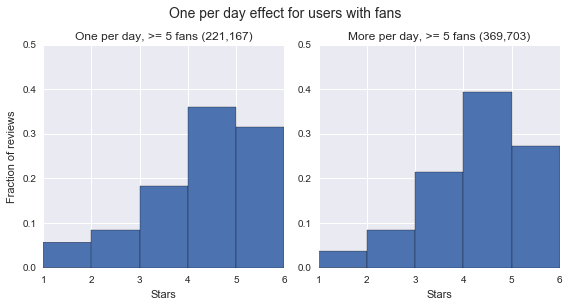
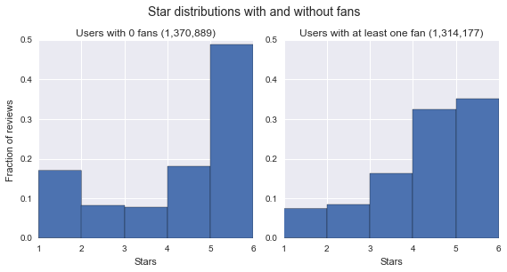
Another interesting effect is what happens when you limit to users with fans (the intuition being that these users may have an influence on other user's predictions). Below to the left, we can see that users with fans tend to give more balanced reviews. Interestingly, when we condition on one per day vs. many per day for users with fans, the extremifying effect of giving only one review per day becomes much weaker. That suggests there are richer and more complicated phenomena underlying the differences in why users give different patterns of stars. You can find more analysis of temporal effects in the notebook here.
Exploring Space
One of the other tasks mentioned in the Netflix Challenge was how dependent a business's success was on just its location. While this was somewhat tangential to the original task of predicting user ratings, we were interested to see what data exploration could reveal and used this to inform whether neighborhood clustering could be a useful predictor in future models.
As a marker of business success , the only really informative column in the businesses dataframe is whether or not the business is still open. In particular, star ratings really aren't a good predictor of whether or not a business is actually successful - we've all seen well-reviewed restaurants go out of business, and McDonald's tends not to have great Yelp reviews but is still one of the most successful businesses of all time.
Then, to investigate this question, we split the restaurants and bars based on those that were still open and those that were closed and then clustered the restaurants using k-means clustering based on their latitude and longitude. While it's true that most cities have a more formal delineation of neighborhoods than this, it should give us a good estimate. We note also that the Yelp data has a "neighborhood" column but that it tends to be unpopulated.
Most notably, we find that among restaurants that are still open, the restaurants outside of the center of the city tend to have a lower star rating. Intuitively, this can be interpreted as suggesting that restaurants that have lower competition tend to stay open despite their lack of relative quality. An even better measure of success might be the time that a restaurant stays open, but this is difficult to determine from the data supplied.
A different interpretation of this result is that the restaurants are of a similar quality but a centralised 'herd' effect helps to raise the reviews of all restaurants in the city center. Whatever the underlying reason that causes this trend, it is worth noting that raw score alone should not be used to make a final prediction (as a 3.1 in one location could actually be as good at a 3.5 in another).
Network Analysis
Restaurants can be viewed as a correlation network based on how similarly users view them. We define two businesses as being positively correlated when users tend to give both businesses the same (or similar) number of stars, and negatively correlated when users tend to rate one business as good but the other as bad. Constructing a network in this way, we aimed to find the most highly-correlated restaurants based on the network structure. When the star-ranking is positively correlated between two businesses, they are connected with a red edge in the business network. When the star-ranking is negatively correlated between two businesses, they are connected with a blue edge. We then calculated Spearman's ranked correlation coefficients for the top-100 frequently reviewed businesses in Phoenix, and applied the PageRank algorithm to infer the importance of restaurants in the network. We then used the PageRank rankings to construct a simple model to predict stars. You can check out the notebook with this analysis here.
Table Showing the 5 Most Highly Connected Restaurants in Phoenix
| Name | Categories | Review Count | Avg. Stars |
|---|---|---|---|
| Lo-Lo's Chicken & Waffles | Soul Food, Waffles, Southern, Restaurants | 1218 | 3.99 |
| Pizzeria Bianco | Italian, Pizza, Sandwiches, Restaurants | 1743 | 3.90 |
| FEZ | Bars, Mediterranean, Nightlife, Lounges | 1093 | 4.16 |
| Chelsea's Kitchen | American (Traditional), Restaurants | 987 | 4.12 |
| St. Francis Restaurant | American (New), Restaurants | 1154 | 3.97 |
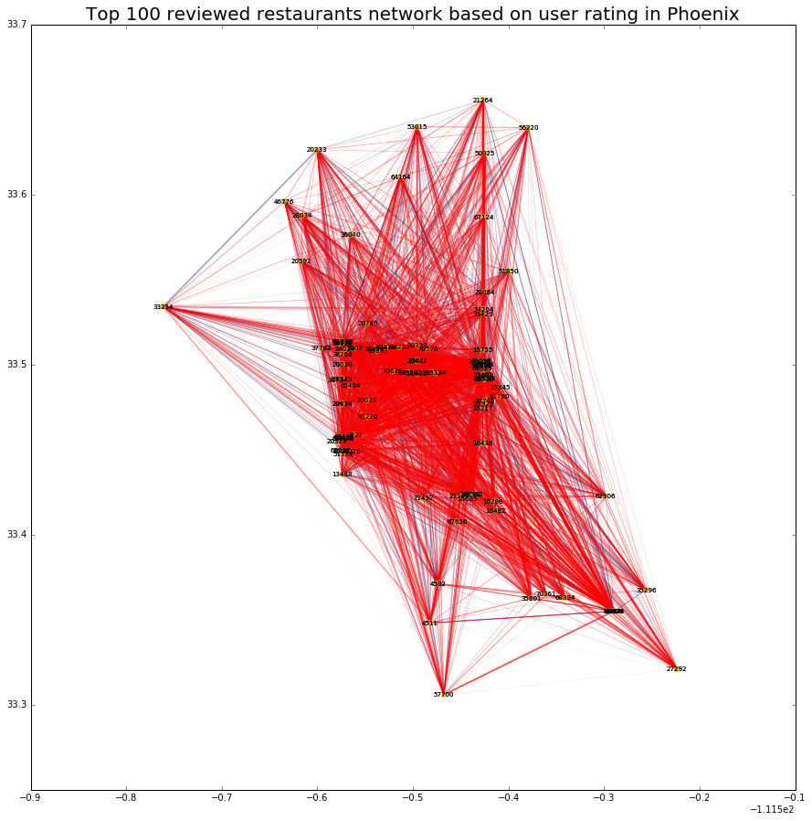
Nodes represent business IDs, and X and Y axes are their longitude and latitude. Degree indicates the total number of edges a node has. The median value was higher in the positive correlation network (63.0) compared with the negative correlation network (28.0), suggesting that there are more restaurants with the similar level of likeness by users in Phoenix.
What is Eigenvector Centrality?
If you consider a random walk over a restaurant network, where at any individual restaurant node at any given time step, you travel to the next restaurant node with probability proportional to the strength of their correlation, then the scores determined by eigenvector centrality will be the relative proportion of time you spend at each restaurant node. This method, made famous for its use in Google's PageRank algorithm, provides an intuitive and computationally tractable way of ranking nodes in general graphs.
Highly connected restaurants in the network (i.e. nodes with more edges) are highly reviewed by users who also reviewed the neighboring restaurants. Thus, the network provides information on how users liked both connected restaurants. To find the "most imporant" restaurants, we calculated their eigenvector centrality in the combined positive and negative network. Eigenvector centrality assigns relative scores to all nodes in the network based on the connectivity of the node and its neighbors. The top 95% highly connected restaurants are shown in the table above.
Baseline Predictors
As a prerequisite to generating personalized recommendations, we first investigate the calculation of baseline predictors. These are predictions for each user and each business that are meant to represent the inherent criticality of the user and quality of the business. The calculation of these predictors should help normalize the data for use in more sophisticated algorithms later, as well as lead to better predictions when we lack data about a new user or business.
The simplest way of using baselines is $$ \hat{r}_{ui} = \mu + b_u + b_i, $$ where \(\hat{r}_{ui}\) is our rating prediction, \(\mu\) is the global mean rating, and \(b_u\) and \(b_i\) are our user and business (or item) baselines, all of which we learn from our training data. Defined in this way, we can use them as a standalone prediction model, although in practice [2] other models are trained on their residuals, or baselines values are determined alongside other parameters in a more complex model trained via an optimization technique.
RMSE - Root Mean Square Error:
We will be referring to Root Mean Square Error (RMSE) throughout the rest of this discussion and so it is a good plan to get you comfortable with the concept. This is our standardized metric for comparing different models as it measures the inherent error that is present between the prediction and the truth. For example, if we have a user that gives a restaurant a score of 3 stars, but we predict that the user would love the restaurant and would give it a score of 5 stars then our model has made a prediction error of 2 stars. The root mean square error metric takes all of these miss-predictions, squares them, averages the squared term and square roots the resulting average. You can think of an RMSE of 1.5 as the model (on average) predicting 1.5 stars incorrectly for every user in either direction.
We'll outline a few of the methods from [2] that we replicated, along with their (baseline) RMSEs on the Phoenix test set. You can see code for the baselines here.
Always Predict The Mean
The most simple baseline is to just predict the mean rating across all users and all businesses in the training set for each rating in the test set: $$ b_u = b_i = 0 $$ This results in an RMSE of 1.354.
Simple Averaging
In this method, we simply compute the baseline for each restaurant or user to be its average deviation from the mean rating $$ b_* = \frac{\sum_{r_* \in R(*)} (r_* - \mu)}{|R(*)|}, $$ where we adopt the convention that \(*\) can refer to either \(u\) or \(i\), \(R(*)\) indicates the set of reviews in our training set given by \(u\) or to \(i\), and \(r_{ui}\) or \(r_*\) is a particular review in our training set. We may further abbreviate \(\sum_{r_* \in R(*)}\) as just \(\sum_*\). With those notation notes out of the way, the RMSE of this method was 1.347.
The Beta Prior Method
This is a method we created, inspired by the homework assignment on movie recommendations. In this method, the baseline for each restaurant or user is defined to be the mode of a Beta posterior distribution, where the two parameters are set based on the "upvotes" and "downvotes" in the training data plus a prior, centered at \(\mu\), whose strength we parameterized:
$$
b_* \sim 1 + 4\cdot\text{Beta}\left(a + \sum_*\frac{r_*-1}{4}, \text{ }b + \sum_*\frac{5-r_*}{4}\right) - \mu
$$
We think of \((r_*-1)/4\), which is 1 for a five-star review and 0 for a one-star review, as an upvote, and \((5-r_*)/4\), which is 0 for a five-star review and 1 for a 0-star review, as a downvote. \(a\) and \(b\) are chosen such that \(a+b\) equals a regularization parameter \(\alpha\) while we require that the Beta mode \(\frac{a-1}{a+b-2}\) equals the global mean \(\mu.\) That gives
$$
a = \frac{(\mu - 1)(\alpha-2)}{4} + 1, \text{ }b = \alpha-a.
$$
For the Phoenix set, we found that the optimal value of \(\alpha\) was \(\approx 8\), which gave us an RMSE of 1.229. You can see the code here.
Note that we had a typo on the poster, in case you're cross-referencing this!
Decoupled Regularized Averaging
The first method outlined by [2] is the following modification of simple averaging. First, we calculate the value of the baseline for a given restaurant by computing the regularized average deviation from the mean for that restaurant. Then when computing similar regularized baseline values for each user we additionally subtract out the baselines we have already calculated for each restaurant in addition to the mean across all ratings. This decoupling process allows us to more accurately model specific user-restaurant interaction: $$ b_i = \frac{\sum_u (r_{ui} - \mu)}{\lambda_1 + |R(i)|}, b_u = \frac{\sum_i (r_{ui} - b_i - \mu)}{\lambda_2 + |R(u)|} $$ For the optimal values we determined for \(\lambda_1\) and \(\lambda_2\) (which were 5.25 and 2.75), we obtained an RMSE of 1.2247.
Least-Squares and the L2 Norm
The second method outlined by [2], which was also used in [3] and many other analyses, is posed as a least-squares problem, where we seek to minimize the sum over all ratings of [rating(user, restaurant) - mean over all ratings - the baselines for the user and rating in question] while using an L2 regularization penalty to push the values of the baselines toward zero: $$ b_* = \text{argmin}\left[ \sum_{u,i} (r_{ui} - \mu - b_u - b_i)^2 + \lambda_3\left(\sum_u b_u^2 + \sum_i b_i^2\right)\right] $$ In [2], the parameters were determined via gradient descent, since the gradient is simple to calculate analytically: $$ \frac{\partial \text{ loss function}}{\partial b_*} = 2\lambda_3b_* - \sum_* 2(r_* - \mu - b_u - b_i) $$ Because our dataset, even limited to Phoenix, was very large (for this method, we needed to estimate 150,619 parameters), the optimization libraries we tried all ran out of memory, so we implemented a simple (and slightly adaptive) version of gradient descent, which we used to find the parameters in a memory-efficient manner (with convergence typically occuring within 200 iterations). For our best \(\lambda\) of \(\approx 4.5\), we obtained an RMSE of 1.2251.
A comparison of the above methods (from the perspective of testing different Beta prior strengths) can be seen here:

Note how much simple averaging overfits, and how the Beta method initially reduces to simple averaging, but approaches the performance of the methods from [2] for the best prior strength values.
Time-Based Baselines
Although the above methods were used in various iterations of the BellKor solution, they obtained their best results from using time-varying baselines (which introduce the first real input data into the problem). In section IIIA of [2], they provide some strong motivation for using time-varying baselines, much of which also applies to the Yelp dataset. In particular, they note that the baseline popularity of movies tends to vary over time (which makes intuitive sense), so instead of a single item baseline \(b_i\), they define an overall baseline \(b_i\) and time-period specific baselines \(b_{i,\text{Bin}(t)}\) corresponding to a particular binning of the full dataset duration.
For users, they didn't find the time-binning method as effective (in part because user reviews tend to be more scattered in time), but they did find a different method of modeling gradual drifts in users ratings over time, as well as incorporating corrections for specific days. One of their most interesting findings was that user behavior differed significantly based on how many reviews that user gave in the same session, and incorporating terms specific to the rounded log of that day-specific "frequency" reduced their RMSE significantly.
These approaches seemed promising to us both intuitively (since, like movies, we expect restaurants to come in and out of fashion over time), and also due to what we discovered in data exploration -- namely, that the prevalence of different ratings had been changing over time, and that there was a significant difference in the behavior of users who rated one business vs. many in a given day.
However, our results weren't quite as good. For the business time binning $$ b_* = \text{argmin}\left[ \sum_{u,i} (r_{ui} - \mu - b_u - b_i - b_{i,y})^2 + \lambda\left(\sum_u b_u^2 + \sum_i b_i^2 + \sum_{i,y} b_{i,y}^2 \right)\right] $$ where \(y \in \{2008,\cdots,2016\}\) now represents the year of the review, we obtained an RMSE of 1.2258 for \(\lambda=6\).
When we attempted to incorporate frequency (number of reviews per day) information into the model, we achieved our best performance with the following model: $$ b_* = \text{argmin}\left[ \sum_{u,i} (r_{ui} - \mu - b_u - b_i - b_{i,f})^2 + \lambda\left(\sum_u b_u^2 + \sum_i b_i^2 + \sum_{i,f} b_{i,f}^2\right)\right] $$ where \(f \in \{0,1\}\) is simply a binary variable indicating whether there were multiple reviews or only one review given, and following [2] we also apply it to the business rather than the user (which we also tried, but to worse results). For \(\lambda = 4.67\), this method actually gave us our best baseline RMSE of 1.2239, which suggests that frequency information is actually meaningful.
However, the reduction in RMSE by including temporal factors is quite small, especially when compared to the dramatic results reported in [2]. Although the most likely explanation for this disparity is that our methods are much less sophisticated, a few possible data-based reasons are that, to begin with, restaurant reviews may be inherently noisier than movie reviews. A movie is identical every time it is watched, but a restaurant experience is always different, and depends on a huge number of independently moving parts. Additionally, the notable temporal effect we noticed -- that reviews given alone on a day tend to be more extreme -- may not be terribly helpful for reducing RMSE using the above method, because if a unknown rating is more likely to be either a 1 or a 5, and we want to represent that by a constant additive factor, then that factor will be pulled in opposite directions. It would be interesting to explore using it more heavily in a classification model that treated ratings as a categorical variable, rather than a numerical one (which might even be more appropriate for the data, given the qualitatively different reasons why people award different numbers of stars).
Once again, the code for all of these methods can be found here, and you can also view the iPython notebook we used to generate these results.
Matrix Factorization
Many of the most successful models in the Netflix Challenge were latent factor models, also commonly known as matrix factorization (MF) models by their usual implementation. In these models, vectors of factors describing users and items are inferred from the sparse data we have for their existing ratings, often using matrix factorization techniques such as singular value decomposition. Once we've inferred user vectors \(p_u\) and item vectors \(q_i\), we can then make a prediction using $$ \hat{r}_{ui} = b_{ui} + p_u^\intercal q_i, $$ where \(b_{ui}\) is a catch-all term for any baseline factors we may or may not have precalculated.
Although we didn't implement any of these models from scratch, we did try three open-source implementations:
- GraphLab Create's FactorizationRecommender
- Surprise's implementation of SVD++
- Vowpal Wabbit's arguably documented matrix factorization mode (for which we wrote a small Python wrapper)
First we tried using them without any of our work on baselines. With a little bit of parameter experimentation, we were able to obtain the following RMSEs:
| Model | RMSE | L1 Penalty | L2 Penalty |
|---|---|---|---|
| Vowpal Wabbit | 1.2362 | 0 | 1e-3 |
| Surprise | 1.2344 | 0 | 2e-2 |
| GraphLab Create | 1.2252 | 1e-5 | 1e-4 |
What's notable is that just using our baseline predictors is sufficient to outperform these models.
We then restricted ourselves to just using GraphLab Create's implementation (because in addition to being the most accurate, it was also the fastest to evaluate), and tried to see if including baselines improved performance. We obtained the following results:
| Baseline Type | Baseline RMSE | MF + Baseline RMSE | MF L1 Penalty | MF L2 Penalty |
|---|---|---|---|---|
| Decoupled + Regularized | 1.2247 | 1.2243 | 1e-4 | 2e-3 |
| Frequency-Aware Least Squares | 1.2239 | 1.2236 | 2.5e-3 | 1.5e-3 |
In both cases, we were able to obtain better performance by combining baselines with MF models (training the MF models to predict the baseline values), but the reductions in RMSE were extremely small.
You can view the iPython notebook with this analysis here.
Limiting User Sparsity
We had been expecting MF models to outperform our baselines more significantly than they did, and we hypothesized that the reason they might not be in this case was that a significant subset of users had only had one review, so many test examples likely had little to no training data for the same user.
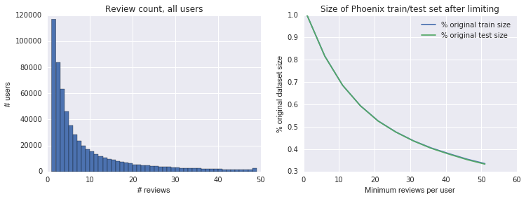
To test this in a simple way, we decided to limit our training and test sets to users with multiple reviews. Below is a plot of the distribution of review count and how data size changed at different minimum review cutoffs. Note that we (somewhat inadvertently) limited based on total review count, rather than enforcing that users appearing in the test set had associated training data, so that condition may only be universally true for large \(n\).
We then trained both baseline and MF models at each cutoff, with a tiny bit of MF parameter searching at each cutoff (though not very much, and none for the baseline models). We were curious to see if MF would start to perform signficantly better than the baseline at high cutoffs. Here are our results (also in a notebook):

First, it's worth noting that all of the methods improve in accuracy as we limit the dataset size, and simple averaging starts to overfit significantly less (since it starts to have much more data to work with). Second, although MF does start to outperform the baseline (by about 0.003) at the highest cutoff, given the lack of regularization parameter optimization, the result doesn't seem very significant.
Interpretable Linear Models
Partially inspired by the prediction methods of the TripAdvisor guest speaker, we created content-based linear models in which we created a matrix with dummies for all of the categorical restaurant information given by Yelp. We then trained a lasso regression model on these predictors with stars as the target variable to determine the most informative categorical predictors. When running this model on new data, we achieved an RMSE of 1.3058 -- lower than the baselines, but interpretable.
Note how "chicken wings", "fast food", and "buffets" are strong predictors of a low rating, whereas "parking lot", "alcohol", and simply "food" are very strong positive predictors of a high one.
We also tried using the baseline correction to retrain a Lasso regression model. We further split the training dataset to be used to build a history of user's reviews. The problem that was incurred here is that we needed to sacrifice half of the training data to purely use in building this history metric, however, this formed a strong predictor and a resultant RMSE of 1.240 was achieved.
Lastly, we used the baseline predictors and half of the training dataset to compute a reasonable baseline transform. This, we then used to create a new predictor (along with all of the other business and user attributes) on the other half of the training set and on the testing test. Again we ran both a Random Forest and a Lasso Regression on this new enlarged dataset. The scores were not improved and critically, the Lasso Regression returned the best cross-validated regularization coefficient when all predictors but the baseline were shrunk to 0. This was in a sense a validation that the baseline work was already maximizing the prediction effort and there was little else left for the other predictors to predict.
Conclusion
User Recommendation Models:
One of the major conclusions of this project is that, because of the sparsity of the user-ratings matrix or otherwise, it's very difficult to do better than baseline rating predictions for the majority of users. In particular, it is nearly impossible to infer much about the users who give only a single rating, and as we see in the time analysis, this single rating may not even be indicative of typical rating behavior - in particular it is likely to be more extreme than usual, likely because a user who gives a single rating is only using Yelp because he or she has had a particularly good or bad experience.
However, with that said, we were able to obtain our best RMSE of 1.2236 using simple versions of many techniques from the BellKor solution -- a matrix factorization model that makes use of time-changing baseline predictors, trained using gradient descent. But, as impressive as it sounds, that result is only about 0.013 points better than our best baseline model performance, and only about 0.001 points better than a baseline predictor-only solution using none of those techniques.
Data Trends:
One of the more enjoyable aspects of this project was the data exploration. In particular, we were able to identify a number of interesting trends in the data sets that either confirmed or made us reconsider previously held notions about consumer opinion of restaurant quality. In the future, we would likely pursue these other aspects of the Yelp Data Challenge, like trying to predict the rise and fall of restaurant trends or whether a good or bad location is enough to cause a business to succeed or fail.
Managing Large Data Sets:
Throughout this project we encountered memory errors and long computation times. Although we found and implemented some workarounds, if we were to continue this work in the future, we would likely switch away from storing our data as in-memory numpy and pandas objects and investigate using databases or remote clusters instead. Sparse matrix data structures provide a good platform for storing and processing these vast review matrices but the computation time required to create them often negated their usefulness down the line.
Thanks for teaching the course (and reading this far)!
References
- The Yelp Dataset Challenge. Accessed 2016.
- Yehuda Koren, The BellKor Solution to the Netflix Grand Prize. 2009.
- Yehuda Koren, Factorization Meets the Neighborhood: a Multifaceted Collaborative Filtering Model. Proc. 14th ACM SIGKDD Int. Conf. on Knowledge Discovery and Data Mining (KDD'08), pp. 426–434, 2008.